View site location on opentopomap
Data since: 07-Nov-2023
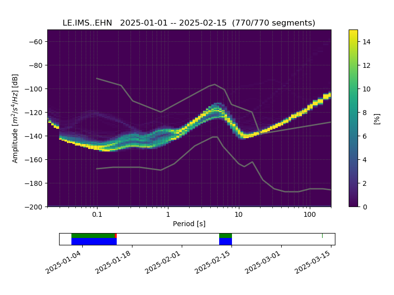
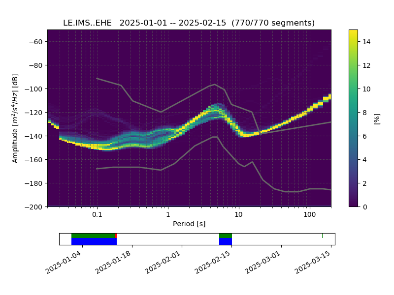
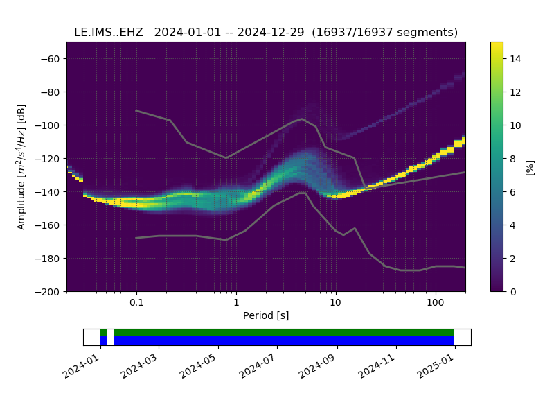
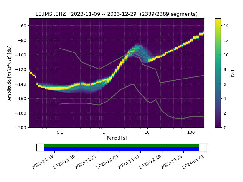
PPSD (Probability Power Spectral Density) of last year, vertical component, transformed to acceleration display.
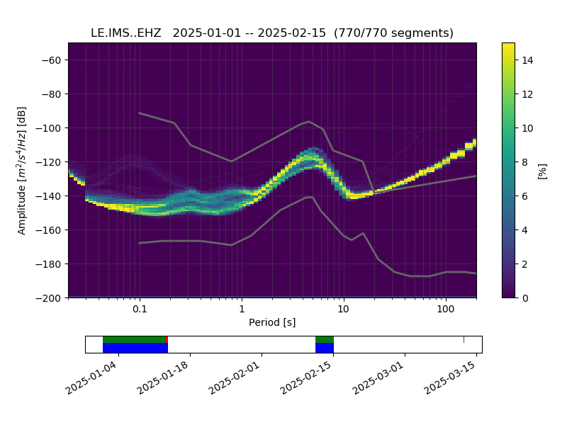
PPSD of vertical component, last year
For other components or years select one of the following links (the figures of the current year are updated daily):
Changes in the PPSD spectra of the vertical component are visualized in the following figure. At all grid frequencies current values are compared with an avarage over a time span of 2 years. Deviations from this mean are color coded: green and yellow colors indicate small deviations, red colors indicate a significant increase in noise power, blue a reduction. Red and blue spots around 10 s reflect natural seasonal noise variations. The PPSD changes figure is updated weekly.

PPSD changes of vertical component, x-axis shows last 365 days (365=yesterday). Upper figure: color coded deviations from average. Lower figure: numerical deviations from average at low (red), mid (pink) and high (blue) frequencies.
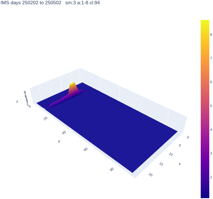
Plot showing the daily and weekly periodicity of averaged anthropogenic noise in the frequency range between 4 and 14 Hz within the last 90 days (in nm/s) in time domain. At some stations the periodicity is masked by wind signals. An interactive figure (turnable and scalable by mouse) and more details describing the content of the figure is available at the anthropogenic noise page. This page needs javascript to be enabled and it takes a few seconds to appear. Please note also the summary page on this topic. This figure is updated daily.
Spectrogram in 2D color display over available time period up to 25 years, vertical component, local wind speed between 3 and 6 m/s (ECMWF model in 10m height). Waveform data are segmented into pieces of 1h length, the resulting PSD values are processed for each grid frequency separately: binned using local wind speed intervals and averaged in time with a median algorithm.
Other components and wind speeds in 2D and 3D display available at the following links:
Please note that the color is scaled for each figure individually, the the scaling with absolute values is shown in the color bar to the right. The 3D figures are slightly smoothed and reduced to make them lighter for handling with javascript. Still it takes a few moments for the 3D figures to show up. All long term spectrograms are updated once a year.
Computes the ratio of two spectral values, one taken at local wind speeds between 0 and 2 m/s and the other taken at speeds between 3 and 6 m/s (see figures above). The spectral values are averaged in time before division. The resulting plot shows spectral elements with an amplitude ratio larger than 1 indicating that these are wind-dependent. Vertical bands in the background result from the saisonal variance of the wind activity. Due to the usage of an interpolation algorithm data gaps apparently disappear.
For viewing all components use links below.
Wind dependent spectra of year ... showing 6 wind bins from 0-2 m/s to 6-12 ms/s (local wind speed from ECMWF model in 10m height). Median-averaged spectral data of different wind bins (same data as used in previous spectrograms) are plotted versus time using different colors. This figure is updated once a year.
For viewing all components use links below.
For data of other years or a comparison with other stations please visit the wind dependent spectra website.
From hourly PSD spectra one frequency is selected and displayed over the whole time span of available data (blue points). A median average curve is computed and plotted in red. Broadband stations will be displayed at frequency 0.15 Hz all other stations at 0.95 Hz. At 0.15 Hz a clear seasonal variation (low in summer, high in winter) should be visible.
For viewing all components use links below.
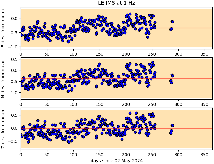
The amplitude stability is checked at a frequency of 0.15 Hz for broadband stations and 1 Hz otherwise. For each of the last 365 days an average PSD amplitude at this frequency is determined and compared with the average of all other stations. The figure shows the deviation from this global average together with the mean (red line) and a tolerance area based on multiples of the standard deviation (orange area). A station with stable amplitudes has all day dots in all components within this range. Trends or steps in this amplitude display may indicate problems with data or metadata. This figure is updated daily.
Correlating signals of teleseismic events between stations reveal possible issues in timing, waveform shape and amplitudes. The x-axis on all diagrams is the event time. The left figure contains the correlation coefficients ranging between -1 and 1. The area between -0.7 and 0.7 is shaded in gray to indicate bad correlation values. The central figure shows the time residuals (in seconds, vertical axis) of the correlation maximum. In an ideal case the values are aligned along the dashed zero line. A mean deviation from zero indicate station corrections in travel time. To be able to display also large residual values the shaded areas at the bottom and on top provide a logarithmic scaling rather than the linear scaling in the central part. Residuals corresponding to low correlation coefficients (below 0.7) have a reduced alpha value appearing less bold in the figure. The right diagram displays the relative amplitude measurements of this station compared to all others on the vertical axis. The dashed line indicates a relative amplitude of 1. The shaded area again indicates logarithmic scaling for large amplitude deviations. Red points result from WWSSN-SP simulations, orange from SRO-LP. Dark blue and light blue show results for horizontal components N and E, respectively, using a KIRNOS simulation. This figure is updated on every new event analysed.
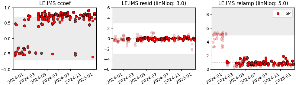
More detailed results of the correlation computations are available at the ftp site of the data center.